equilibrium

library(tree)

library(parallel)

run <- function(seed_rain_in, p, schedule) {
  p$seed_rain <- seed_rain_in
  run_ebt(p, schedule)$seed_rains
}

run_new_schedule <- function(w, p, schedule=NULL) {
  p$seed_rain <- w
  res <- build_schedule(p, schedule)
  unname(attr(res, "seed_rain")[,"out"])
}

Try to establish what the equilubrium seed rain is.

p <- ebt_base_parameters()

p$add_strategy(new(Strategy, list(lma=0.08)))

p$seed_rain <- 1.1

1: Approach to equilibrium:

res <- equilibrium_seed_rain(p)

## 1: Splitting {27} times (141)
## 2: Splitting {10} times (168)
## *** 1: {1.1} -> {25.8} (delta = {24.7})
## 1: Splitting {37} times (141)
## 2: Splitting {21} times (178)
## 3: Splitting {12} times (199)
## 4: Splitting {8} times (211)
## *** 2: {25.8} -> {22.11} (delta = {-3.69})
## 1: Splitting {1} times (219)
## *** 3: {22.11} -> {22.26} (delta = {0.1473})
## *** 4: {22.26} -> {22.25} (delta = {-0.006802})
## *** 5: {22.25} -> {22.25} (delta = {0.0003452})
## *** 6: {22.25} -> {22.25} (delta = {-1.673e-05})
## *** 7: {22.25} -> {22.25} (delta = {8.111e-07})
## Reached target accuracy (delta 8.11121e-07 < 1.00000e-05 eps)

seed_rain_eq <- unname(res[["seed_rain"]][,"in"])

schedule1 <- res[["schedule"]]$copy()

Sanity and time check

system.time(delta <- run(seed_rain_eq, p, schedule1) -
            unname(res[["seed_rain"]][,"out"]))

##    user  system elapsed 
##   4.644   0.014   4.782

delta

## [1] 0

Plot the approach:

approach <- t(sapply(attr(res, "progress"), "[[", "seed_rain"))

From a distance, these both hone in nicely on the equilibrium, and rapidly, too.

r <- range(approach)

plot(approach, type="n", las=1, xlim=r, ylim=r)

abline(0, 1, lty=2, col="grey")

cobweb(approach, pch=19, cex=.5, type="o")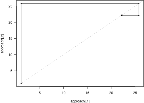

Zoom in on the last few points:

r <- seed_rain_eq + c(-1, 1) * 0.03

plot(approach, type="n", las=1, xlim=r, ylim=r)

abline(0, 1, lty=2, col="grey")

cobweb(approach, pch=19, cex=.5, type="o")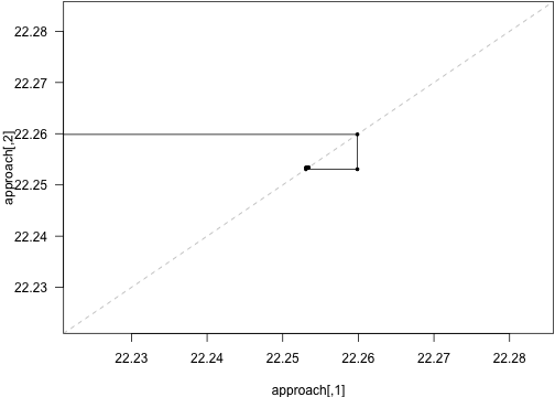

Zoom in on the last few points to see where the insability kicks in:

r <- seed_rain_eq + c(-1, 1) * 0.000003

plot(approach, type="n", las=1, xlim=r, ylim=r)

abline(0, 1, lty=2, col="grey")

cobweb(approach, pch=19, cex=.5, type="o")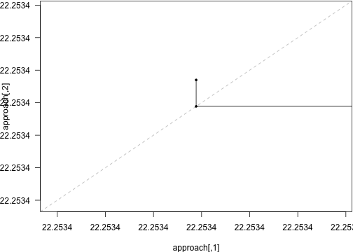

2: Near the equilibrium point:

Then, in the vinicity of the root we should look at what the curve actually looks like, without adaptive refinement.

dr <- 2 # range of input to vary (plus and minus this many seeds)

seed_rain_in <- seq(seed_rain_eq - dr,
                    seed_rain_eq + dr, length=31)

seed_rain_out <- unlist(mclapply(seed_rain_in, run, p, schedule1))

fit <- lm(seed_rain_out ~ seed_rain_in)

Here is input seeds vs output seeds:

plot(seed_rain_in, seed_rain_out, xlab="Incoming seed rain",
     ylab="Outgoing seed rain", las=1)

abline(0, 1, lty=2, col="grey")

abline(fit, lty=2)

cobweb(approach)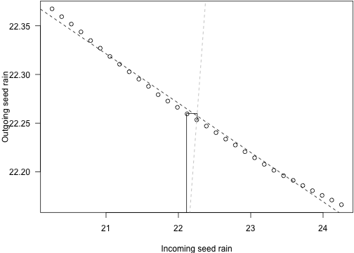

See instability.R for more exploration of this:

plot(seed_rain_in, resid(fit),
     xlab="Incoming seed rain", ylab="Residual seed rain",
     las=1, pch=1)

abline(h=0, v=seed_rain_eq)

4. Global function shape

seed_rain_in_global <- seq(1, max(approach), length.out=51)

This takes quite a while to compute.

seed_rain_out_global <-
  unlist(mclapply(seed_rain_in_global, run_new_schedule, p))

This is pretty patchy, which is due to incompletely refining the cohort schedule, I believe. Tighten schedule_eps to make the curve smoother, at the cost of potentially a lot more effort.

plot(seed_rain_in_global, seed_rain_out_global,
     las=1, type="l",
     xlab="Incoming seed rain", ylab="Outgoing seed rain")

abline(0, 1, lty=2, col="grey")

abline(fit,  lty=2)

cobweb(approach, lty=3)

5. Multiple species at once:

p <- ebt_base_parameters()

p$add_strategy(new(Strategy, list(lma=0.08)))

p$add_strategy(new(Strategy, list(lma=0.15)))

p$seed_rain <- c(1.1, 1.1)               # Starting rain.

res <- equilibrium_seed_rain(p)

## 1: Splitting {10,22} times (141,141)
## 2: Splitting {0,9} times (151,163)
## 3: Splitting {0,3} times (151,172)
## *** 1: {1.1,1.1} -> {17.46,18.12} (delta = {16.36,17.02})
## 1: Splitting {19,25} times (141,141)
## 2: Splitting {5,27} times (160,166)
## 3: Splitting {0,12} times (165,193)
## 4: Splitting {0,3} times (165,205)
## *** 2: {17.46,18.12} -> {16.83,12.54} (delta = {-0.6296,-5.578})
## *** 3: {16.83,12.54} -> {16.84,12.53} (delta = {0.01047,-0.008564})
## *** 4: {16.84,12.53} -> {16.84,12.53} (delta = {-0.0003415,-0.0003512})
## *** 5: {16.84,12.53} -> {16.84,12.53} (delta = {9.71e-06,1.234e-05})
## *** 6: {16.84,12.53} -> {16.84,12.53} (delta = {-2.769e-07,-3.537e-07})
## Reached target accuracy (delta 3.53698e-07 < 1.00000e-05 eps)

seed_rain_eq <- res[["seed_rain"]][,"out"]

progress_seed_rain <- lapply(attr(res, "progress"), "[[", "seed_rain")

approach <- lapply(seq_len(p$size), function(i)
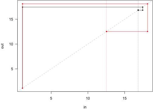
                   t(sapply(progress_seed_rain, function(x) x[i,])))

From a distance, these both hone in nicely on the equilibrium, and rapidly, too.

r <- range(unlist(approach))

plot(approach[[1]], type="n", las=1, xlim=r, ylim=r)

abline(0, 1, lty=2, col="grey")

cols <- c("black", "red")

for (i in seq_along(approach)) {
  cobweb(approach[[i]], pch=19, cex=.5, type="o", col=cols[[i]])
}

abline(v=seed_rain_eq, col=1:2, lty=3)