NonlinearEquations.jl: A tool for automatically differentiating systems of nonlinear equations

Description

NonlinearEquations.jl is a Julia module that includes automatically differentiates systems of nonlinear equations, producing sparse Jacobians. Consider a simple example:

import NonlinearEquations
import SparseArrays#the code generated by NonlinearEquations will require SparseArrays

@NonlinearEquations.equations function f(x, a, b)
	NonlinearEquations.setnumequations(2)#there  will be 2 equations
	NonlinearEquations.addterm(1, a[1] * x[1])#add a term to the first equation
	NonlinearEquations.addterm(1, b[1] * x[2])#add another term to the first equation
	NonlinearEquations.addterm(2, a[2] * x[1] + b[2] * x[2])#add a couple terms to the second equation at once
end

This code defines a system of two linear equations. The notation NonlinearEquations.setnumequations(N) tells NonlinearEquations the number of equations. You can think of each equation as starting out as 0=0. We can then add terms to the left hand side of the equations with the notation NonlinearEquations.addterm(equation_number, term). Note that any code outside the NonlinearEquations.addterm is not differentiated when computing Jacobians, so care must be taken to include everything that should be differentiated in there. The macro @NonlinearEquations.equations translates this description of the equations into a series of functions:

x = randn(2)
a = randn(2)
b = randn(2)
#f_residuals basically plugs the numbers into the equations and sees how they differ from 0
@show f_residuals(x, a, b) == [a[1] * x[1] + b[1] * x[2], a[2] * x[1] + b[2] * x[2]]
#f_x computes the jacobian of f_residuals with respect to x
@show f_x(x, a, b) == [a[1] b[1]; a[2] b[2]]
#the focus of the package is on large, sparse systems of equations, so the type of f_x(x, a, b) is a sparse matrix:
@show typeof(f_x(x, a, b))
#f_a computes the jacobian of f_residuals with respect to a
@show f_a(x, a, b) == [x[1] 0; 0 x[1]]
#f_b computes the jacobian of f_residuals with respect to b
@show f_b(x, a, b) == [x[2] 0; 0 x[2]]

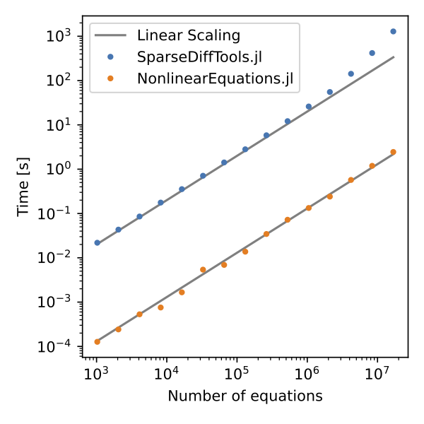
NonlinearEquations can be viewed as an alternative to SparseDiffTools. NonlinearEquations uses a source-to-source translation approach, whereas SparseDiffTools uses a graph coloring approach. This means the "time to first Jacobian" is faster and appears to scale better for NonlinearEquations than SparseDiffTools:

The above comparison was for the Laplacian example in SparseDiffTools' README. To implement this example with NonlinearEquations, we would write:

@NonlinearEquations.equations function gw1d(h)
	NonlinearEquations.setnumequations(length(h))
	NonlinearEquations.addterm(1, -2 * h[1] + h[2])
	for i = 2:length(h) - 1
		NonlinearEquations.addterm(i, h[i - 1] - 2 * h[i] + h[i + 1])
	end
	NonlinearEquations.addterm(length(h), -2 * h[end] + h[end - 1])
end

The examples illustrate more complex behavior. It is also used in the DPFEHM subsurface flow simulator.

License

NonlinearEquations.jl is provided under a BSD style license. See LICENSE.md file for the full text.

This package is part of the Orchard suite, known internally as C20086 Orchard.

Author

Daniel O'Malley, [email protected]